Upon initial look, the Smith chart appears to be quite complicated. Although the basis for the chart is deeply rooted in complex variable theory, you do not have to be a graduate-level mathematician to appreciate and have a solid working knowledge of the chart. While calculation methods can be performed via computer or calculator with a greater degree of accuracy, the Smith chart still remains a venerable and useful tool for the RF engineer.
One good working definition of the Smith chart is that it is simply a graphical calculator for normalized impedance and associated RF parameters. When impedance is normalized, it is related to a reference value as a multiple. For obvious reasons values of 50 and 75? are the most common bases utilized. In the simplest form, if 50? is our reference value, then 50, 100 and 25? normalized would become 1?, 2? and 0.5? respectively.
Impedance is a measure of the opposition of the flow of current in an alternating current circuit. It is the complex sum of the resistance and reactance components, and thus, in ac circuits describes not only the ratio of voltage and current, but also the relative phase angles. Impedance can be written a number of different ways; however, you probably will see the Cartesian forms below more often than not.

The difference in these two equations results from the flavor of reactance. Inductive reactance is defined as positive, while capacitive reactance is negative. The reason for the sign change is how voltage and current are related in inductors and capacitors. Recall “ELI the ICE man” and that voltage leads current by 90 degrees in an inductor and vice-versa in a capacitor. Finally, note we are only considering positive resistance values. Negative resistance values do occur with some regularity in directional antenna systems; however, they are not manifested in passive circuits and not represented on the basic Smith chart as we will infer shortly.

THE DETAILS
The Smith chart (Fig. 1) is constructed from three families of circles. The first family of circles is tangent to a point on the right side of the outer circle along the center horizontal line. Each of these circles has a constant normalized resistance value. As one moves along any particular circle, the resistance value of the impedance will remain constant, but the reactance will vary.
The second family of circles is that of constant reactance, which are tangent to the same point as the constant resistance circles but are rotated clockwise or counter-clockwise by 90 degrees. These circles form what appear to be arcs on the basic chart with positive or inductive reactance lying above the center line and the converse for capacitive or negative reactance. Reactance is a frequency dependent quantity and can be calculated by the following:

The third set of circles is not normally visible on typical versions of the chart save for one element. These circles form the constant reflection coefficient circles and are concentric radiating out from the center of the chart. Although not strictly correct, these circles can also be thought of as constant VSWR circles because of the relationship between the reflection coefficient and VSWR.
The reflection coefficient varies from a maximum of -1 through 0 to 1. A perfect short is realized by a reflection coefficient of -1, while 1 represents a perfect open, and zero a perfect match. Since a perfect open or short is not usually realized, it is usually more accurate to represent the reflection coefficient, denoted by G, with a phase angle.
The reflection coefficient is then related to the load impedance (?L), characteristic impedance (?0) and VSWR (S) through the next two equations. The absolute value bars in the second equations are necessary to force the VSWR value to a positive number.

A perfect short is nothing more than an impedance of 0?, while a perfect open would be an impedance of infinite ?. As we move from the right side of the chart to the left side, the normalized resistance values decrease from infinity to zero. Thus a perfect open is represented by the point along the horizontal axis on the right side of the chart while a short is the corresponding point on the left side of the impedance chart.
Both of these locations represent a reflection coefficient with a magnitude of 1, so the outer circle of the Smith chart corresponds to a reflection coefficient magnitude of 1. A wave encountering an open circuit is reflected back in phase, while a short is 180 degrees out of phase. So we can see that rotating around the outer ring of the chart relates to the resulting phase shift, and we are able to plot points and directly read the phase shift.
The locations on the outer ring of the chart up and down from the center location, which has an impedance of 1+j0?, the reference value, are a 90-degree phase shift. These locations intersect the 0? resistance circle at +j1 and -j1?, resulting in normalized impedances of 0+j1 and 0-j1?. These are an inductor and capacitor respectively and correspond to the known phase relationship between voltage and current in these components.
There is also a scale for the transmission coefficient, which is the complex sum of 1 plus the reflection coefficient. It is not as widely used as the reflection coefficient. Outward from these two scales are the wavelength scales, used in transmission line calculations. They show that one full rotation around the chart corresponds to one-half wavelength.
Below the chart in Figure 1 there are several radial scales. These scales function as rulers, and can be utilized to make measurements based on items already illustrated on the chart. Typically included are scales for SWR, attenuation, return loss, and transmission and reflection coefficients.

A CALCULATOR
Calculations may be simplified using a ZY chart (Fig. 2). On the ZY chart, the impedance Smith chart is overlaid by its admittance Smith chart, which is created by rotating the impedance chart by 180 degrees. Addition of components in series moves the impedance along a constant resistance circle, while shunt or parallel addition moves the impedance along a constant conductance circle, which is the analog to the resistance circle. With a T or pi configuration, nearly any impedance can be matched to another.
Even when not performing design calculations, the Smith chart provides an excellent method to visualize issues with antenna systems. A simple sweep may illustrate a greatly elevated VSWR. This measured quantity, flat across a range of frequencies, certainly demonstrates the presence of an issue with the system; but where is it located? From a Smith chart plot a relative location may be discerned. If the plot shows large diameter circles centered on the midpoint, then the impedance mismatch is distant from the generator. If the trace results in a compact circle slid off center, then the reflection is closer to the transmitter. In an ideal world, antenna systems would closely approximate a dot in the center of the chart.
For almost 75 years the Smith chart has been a mainstay of RF engineers. Its construct really is quite remarkable, and its ease of use is one reason for its continued relevance in today”s world of calculators and computers.
Ruck is a senior engineer with D.L. Markley and Associates, Peoria, Ill.