In an earlier article we discussed microwave theory for STLs. We discussed factors on which we have some influence: antenna size, transmitter power, type (and associated loss) of transmission lines, etc.
Now let’s consider aspects of the microwave system over which you have no direct control but can predict and work around using accumulated knowledge.
To review, we have learned that there is no direct “loss” due to distance, it’s just that as we move farther from the source terminal, the signal is more diffuse, and therefore, you can capture only a smaller sample.
However, that’s loss in “free space,” which is nothing like the real world. In our world, we have atmospheric disturbances, temperature inversions (which affect “K Factor,” to be discussed later) as well as interference from other sources, destructive signal polarity inversions when a path is over a body of water, among other concerns.
Among the worst issues an engineer may experience with the microwave path, aside from equipment failure, are interference from another transmitter (sometimes at seemingly random times); atmospheric effects such as tropospheric ducting, temperature inversions or polarity reversal of the wave front due to a reflective surface; and objects inserted into the path without prior knowledge such as a new office building.
So we open a toolbox of mitigation methods that are proven to be effective in the design of microwave systems.
Types of diversity
Frequency Diversity: The idea here is to have more than one frequency (or “channel”) in the system design (here by “system,” I mean the entire collection of transmitters, transmission line, antennas, receivers, filters, isocouplers, etc. that comprise your design as a whole).
This type of diversity, implemented properly, provides for robustness. If one channel is experiencing atmospheric anomalies, the other channel(s) may not be so affected.
In the section of 47 CFR Part 74 that deals with rules for 950 MHz STL systems, the channel spread is likely not enough to materially be of use for this type of diversity (that is to say, the entire channel spread is likely to be affected by the self-same disturbance). However, this can still be of good use if there is an interference issue that may affect only one channel, and not another.
Use of an entirely different band, such as 6, 11 or 23 GHz along with a 950 MHz band radio, can be of tremendous benefit by virtue of frequency diversity (this also is a form of technological diversity, to be covered later).
Hawaii suffers from periodic destructive interference during military RIMPAC activities, which lead to unusable 950 MHz links. The “price of freedom,” we are told. In this case, multiple 950 MHz channels are affected.
Space Diversity: Here, the aim is to separate two receive antennas in such a manner as to receive the transmitted signal via multiple paths with some vertical separation. Empirically, a vertical separation of some 200 wavelengths has proven effective. It just so happens this works out to about 200 feet at 950 MHz. So, if you have a receive antenna (which we’ll call the “main antenna”) at 700 feet AGL on the tower, then another antenna (“aux. antenna”) might be at 500 feet of elevation.
I had such an arrangement in Orlando, which performed very well during early morning temperature inversions during which the transmitted signal was diverted downward. I would observe the receiver signal connected to the main antenna begin to drop rapidly while at the same time, the received signal of the receiver connected to the aux. antenna would rise.
In this case, the RSSI as indicated on the receiver connected to the main antenna, which normally would hover around 1100 µV, would drop below 200 µV! This form of diversity worked very well in this system. We’ll discuss the cause of this shortly.
Technological Diversity: This method is my personal choice for almost ultimate robustness. Here, we mix technologies to achieve almost 100% reliability.
Several choices are available to us in 2023. For example, we can use a 950 MHz STL and an audio over IP device such as an Intraplex IP100/200 or a Comrex Bric. Another option is a 6 GHz data link (using an IP200 as the audio codec) as well as a 950 MHz link (a form of frequency diversity discussed above). Further, dedicated fiber from the studio to the transmitter site is an almost ultimate solution.
From a fault tolerance standpoint, if the redundant, diverse systems each have “5 nines” reliability or 99.999% uptime, this means the probability of failure is 1–0.99999 or 0.00001.
This implies the probability of both systems failing at the same time is a remote 0.0000000001 or 1 in 10 billion.
Propagation and path
Now let’s focus on propagation and the path itself.
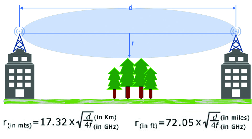
In general, we need a clear, line-of-site path from the microwave transmitter to the receiver antenna (clear of obstacles). We determine this using a terrain profile by using Google Earth or other suitable software. From this we can plot the “Fresnel Zone” (pronounced “Fray-nell”). See Fig. 1.
The formula for calculating the Fresnel Zone is:
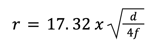
- r = radius in meters
- d = distance in km
- f = frequency in GHz
Typically, 40% intrusion by an object (this was empirically derived) into the Fresnel zone is acceptable, so one can use 0.6 as a constant multiplier. Any further intrusion into the zone is considered a grazing path. If under those circumstances the path has line of site considering the intrusion, add 6 dB to the free space attenuation to compensate.
Reflections and Brewster’s angle
It is well known that microwave paths that traverse bodies of water (lakes, bays, etc.) can be problematic due to the incident wave striking the water surface and thence being reflected out of phase or reversed in polarity. A larger fade margin and a form of diversity are often the only remedies available to the design engineer.
Brewster’s angle is an advanced topic, but for our purposes there exists an angle at which the incident wave is partially refracted into the water and polarized in the reflected wave because of the difference in density of the air/water interface. This can cause a wave front to the receive terminal being compromised by a polarized wave not of the same polarity as that of the transmitted signal.
K factor and “Flat Earth”
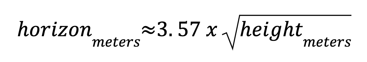
K factor is a relationship of the radio horizon to the true earth radius as a result of tropospheric bending and generally considered to be 4/3 or 1.33. the distance under these conditions is given by:
However, normal isn’t always the case. During temperature inversions in which the overlying air layer is warmer and therefore less dense (common on summer early mornings after the earth has cooled more than the overlying air), K factor can become 1.00, which is known as the “flat earth condition” in which the wave front can travel for a very long distance.
This phenomenon also can lead to FM stations hundreds of miles away booming into your market, inspiring your PD, OM or GM telling you that there’s “something wrong with our signal” or “The station in Colorado must be running ‘super high power,’ call the FCC.”
Generally these issues clear up around 10 a.m. after the sun warms the ground and atmospheric conditions normalize. I experienced this particularly in Central Florida during the summer months.
Knife-edge diffraction
When I was working in Southern California a few years ago, we had a site on a windfarm in Tehachapi (wind turbines by the hundreds) to which the previous engineer attempted a 950 MHz “shot” from the Mojave “main studio.”
No way in the blue blazes would an actual engineer even have attempted this system given the terrain blockage (see Fig. 2). Yet against all odds, it worked after a fashion; the RSSI as indicated by the receiver would vary wildly from 150 to 300 µV continuously (think of a VU meter), but by running the STL system in mono, the system produced a marginally usable audio source.
The only plausible explanation I and my knowledgeable colleague Doug Irwin could come up with is the phenomenon of knife-edge diffraction.
Fig. 3 is the idealized depiction of a knife-edge diffraction scenario. This is the same phenomenon that allows you to hear sound from around the corner of a building (even in absence of reflective surfaces (remember, 1 Hz to beyond X rays are all on the EM spectrum).
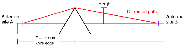
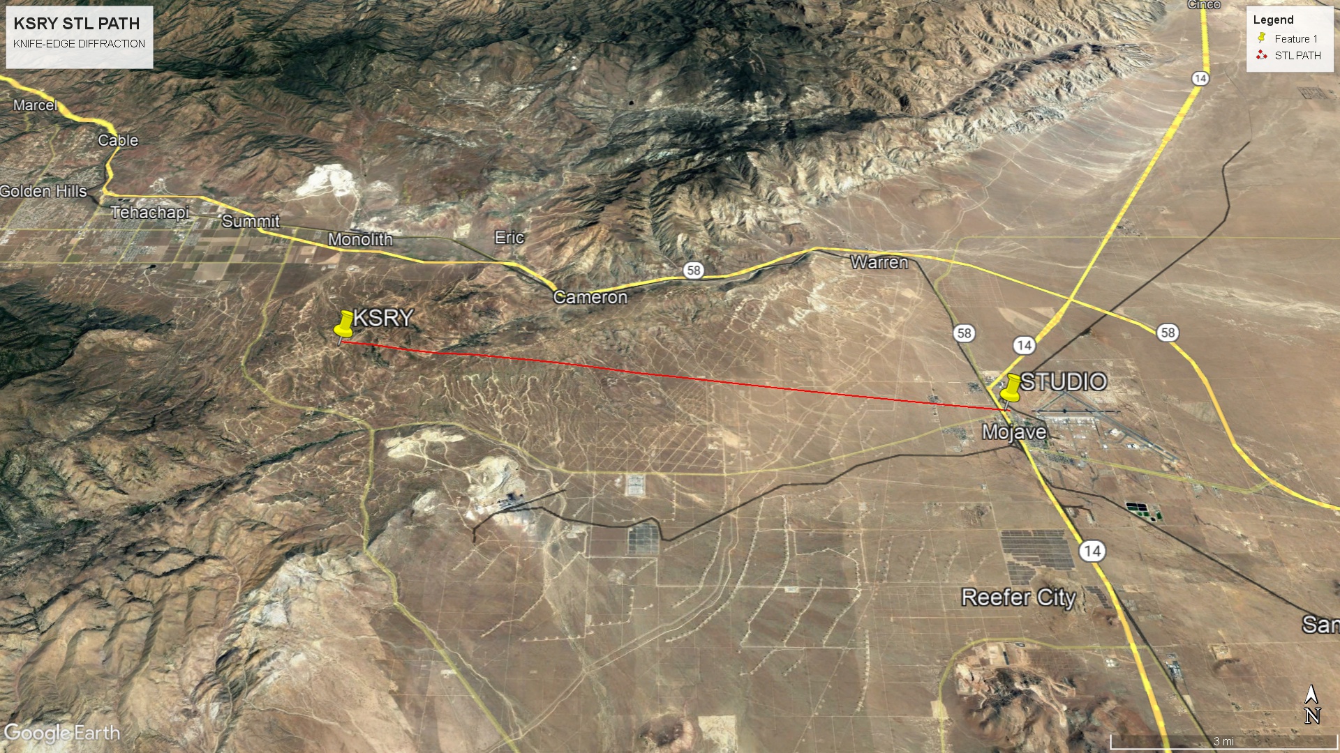
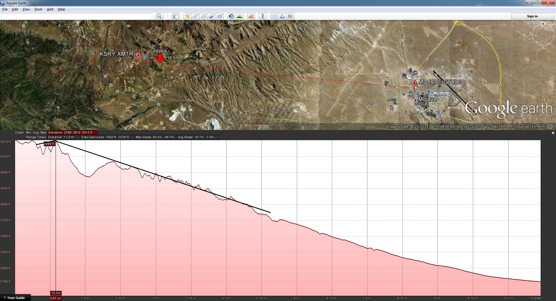
Fig. 4 shows the KSRY path plane view.
Note that the STL transmitter in Mojave is at the extreme right of the illustration and the KSRY site (receiver) is at the extreme left. Note the “knife edge” peak less than a mile from the receiver. This is well beyond a grazing path!
Conclusion
The proper design of a microwave system requires some minimum knowledge of the topics we’ve discussed. Fortunately, a multitude of online calculators exist to assist you. Even with the aid of such calculators, you can make better use of such helpers if you have a basic understanding of the entire system.