Let’s say a corporate engineer or a consultant is coming to your station to diagnose and repair a problem using an RF spectrum analyzer. This would be a great time to schedule a meeting with your local Society of Broadcast Engineers chapter. They and you could learn about these tools.
While you are at it, use the analyzer on other parts of the facility like STL, AM and FM transmitters. If you are the one demonstrating the analyzer, you will find yourself learning in the process of teaching.
Don’t confuse an analyzer with an oscilloscope, which I have referred to a number of times since we published an article titled “Your Scope Is a Tool for All Seasons” in January 2013.
Oscilloscopes display electronic signals in a time versus amplitude format. A dot, sweeping across a screen, will go up or down as it displays audio or RF voltages.
Think of an RF spectrum analyzer as a radio with a slide rule dial where the lower frequency might be 88 MHz and the upper end at 108 MHz. It is a marvelous tool for seeing RF across the entire FM band.
Normally we analyze smaller pieces of the RF spectrum to see greater detail. Think of this technology as creating a “window” into the world of radio frequencies. You can see what and how much is happening on every frequency.
Troubleshooter
I remember receiving a phone call from a station owner saying she could hear her FM at three spots on the dial. My first response was, lucky you, but my next was, I will be right over with my spectrum analyzer.
Sure enough, the station was broadcasting on three frequencies. I had seen this before and was prepared.
Two electrolytic capacitors on the power amplifier board of the station’s FM exciter had dried out, allowing signal spurs, each about 250 kHz from the licensed frequency. After we replaced the capacitors, the spectrum analyzer was the perfect tool for checking the station’s signal. Tuning around with a receiver would have been another method, but there could be other problems and would not confirm that the station’s signal was FCC legal.
Fig. 1 shows an Agilent N9340B Handheld Spectrum Analyzer, not in current production but at eight pounds showing that an analyzer can be carried easily into the field. Anritsu made a similar model.
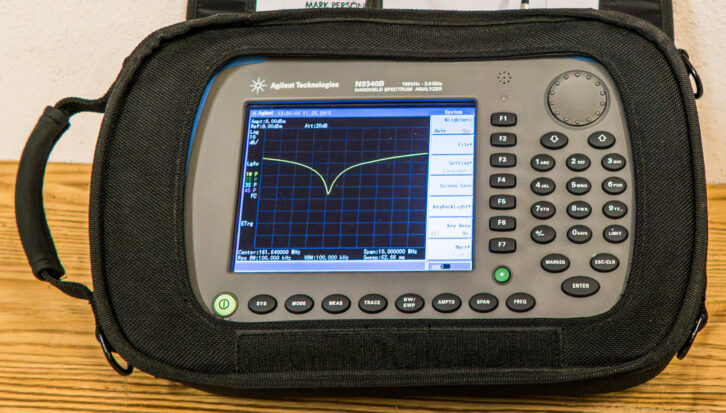
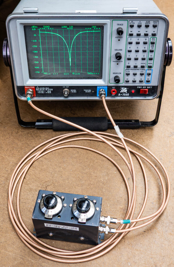
Fig. 2 is an IFR A-7550 RF Spectrum Analyzer, less portable at 28 pounds. This was cutting-edge technology in the 1980s. It is shown verifying a notch filter characteristic. The goal is for the filter to notch out a station’s frequency carrier and therefore extend the dynamic range of a station measurement beyond the analyzer’s 80 dB. The Agilent and IFR were $15,000 instruments back in the day.
More recent analyzer systems are much less expensive and consist of a notebook computer connected to a small box. The computer runs the box and provides a graphical display. Today we are returning to a one-box solution because the cost of an analyzer is often around $1,000.
Occupied bandwidth
Years ago, the FCC required audio performance measurements, with the hope that clean audio was also an indicator of spectral purity. RF spectrum analyzers now provide a way to prove that a station is using a licensed piece of the dial without causing problems to other stations up and down the dial.
Fig. 3 is a spectrum analyzer’s FM display. The left to right frequency span, in this case, is 2 MHz; you can see the FM dial from 105.1 to 107.1 MHz. The red lines are the FCC occupied bandwidth limits, known as the mask. As you can see, this station just barely passes the test.

Fig. 4 is looking at an AM station on 1380 kHz. The display is 200 kHz wide, starting at 1280 kHz and going to 1480 kHz, with 1380 in the middle.
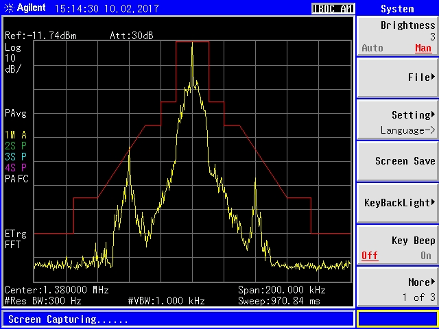
A station on 1340 kHz (two divisions left of 1380) just peeks above the red mask, but that has nothing to do with the 1380 signal under test. However, as you can see, the 1340 and 1380 mix to create a new signal at 1420 kHz. Fortunately, it is below the mask, so it is FCC legal.
When the 1380 transmitter is turned off, the 1380 and the 1420 signals disappear, leaving just 1340 kHz. This on-off testing is often used to prove which signals come from where. If the 1420 kHz mix product was above the red mask line, a filter would be needed to attenuate the 1340 kHz signal, at the 1380 transmitter, so the 1420 mix would be less.
Fig. 5 is a 6.5 MHz wide sweep around 105.3 MHz. Portions of the sweep go above the red mask at 103.7 and 104.5 MHz. Later in this test, the 106.5 transmitter was turned off and those two signals remained. This proved those were other stations on the dial.
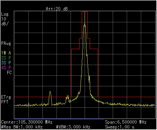
It is rare that a spectrum analyzer sweep shows just the station of interest. FM stations and translators are popping up everywhere and it is wise to check stations on a regular basis, especially if you know that a new one was built within a few miles.
Return loss
Most transmitters have forward and reflected power meters. But that only applies to the frequency of operation.
A spectrum analyzer, with a return loss bridge, can look at the station’s frequency and nearby portions of the spectrum to see where antenna reflected power is lower or higher. The analyzer needs a built-in tracking generator in order for this to work. Think of this arrangement as a poor-man’s network analyzer.
Some newer transmitters have displays to show antenna characteristics at and around a station’s frequency. It is great technology at our fingertips.
Fig. 6 shows a spectrum analyzer connected to a return loss bridge. If the bridge sees a 50-ohm load, the loss from its input port to its output port will be high, causing the displayed sweep to be lower on the screen. If the bridge is connected to an antenna, it will show where the antenna looks most like 50 ohms.
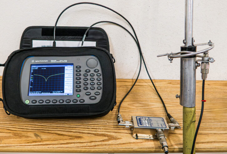
Antennas work best at one frequency. Adjusting the antenna hardware for best match to a transmitter is easily performed this way. As shown, this test setup was used when adjusting a 160 MHz remote broadcast antenna. The same test can be used on an FM broadcast antenna.
Stub traps
Let’s say you build a shorted quarter-wave stub trap to protect an FM exciter’s power amplifier from a potential arc in a vintage tube transmitter. I described one in a Radio World article, “Prevent Transistor Failures With Science,” in May 2013.
That technology is just as valid today. The stub is on one side of a T connector at the output of an FM exciter, or even the output of a full-power transmitter. Science tells us that shorting the center to the outer conductor of a coaxial cable will be electrically invisible if the short is one-quarter wavelength down the line at the frequency of interest. The best part is that it is a DC short to stop voltage spikes. In the case of the FM broadcast band, a shorted stub might be 20 to 30 inches long. Length depends on frequency and velocity factor of cable used.
You don’t just install one without testing first. Fig. 7 shows a return loss sweep of a stub at 97 MHz. The 25 dB dip in the middle is the same as 1:1.12 VSWR.

Analyzers
Not all RF spectrum analyzers are created equal. There are cost vs. performance tradeoffs. Just because an analyzer can look at the frequencies you want to see, doesn’t mean it is good enough for doing FCC required measurements. For instance, an analyzer must have a 300 Hz resolution bandwidth filter for annual AM NRSC measurements. That means it employs a narrow RF filter as it is sweeping across the frequencies of interest.
An analyzer needs to have at least 80 dB of dynamic range between the top of the screen and the bottom to view and certify that unwanted noise and spurs from a 5 kW or greater transmitter is FCC legal. The number is 73 dB at the 1 kW level. That means the noise floor in the analyzer must be sufficient to prove a station is in compliance. Any analyzer you use will need to have a way to output its displays for documentation in an FCC report.
What’s the right model for you? Shop with care. In general, higher cost means more accurate measurements. But learn from someone who has experience in using an analyzer; and purchase one with a money-back guarantee in case the instrument is not right for you or your application.
Learning something new is a good way to grow in broadcast engineering. It makes perfect sense.
The author wrote recently about his visit to Trans World Radio’s “Shine 800 AM” on Bonaire.
Comment on this or any article. Write [email protected].