Calculating STL Fade Margin
Nov 1, 2010 8:53 AM, By Jeremy Ruck, PE

Broadcast auxiliary facilities, and STL systems in particular, tend to get relegated to the back burner. Many times this equipment is glossed over in day-to-day operations, and usually winds up being one of the latter concerns in studio relocation. Understanding the mechanics of your RF program delivery system, and maintaining a keen grasp of the associated fade margin can go a long way to diagnosing the rare, but ultimately problematic impact path failure can have.
In a nutshell, the fade margin is the difference between the received signal level at the input to the receiver and the sensitivity of the receiver. Typically this quantity is expressed in decibels. The higher the number, the more reliable the path.
Creating a path
When analyzing or designing a path, the first step is to ensure the path is viable. Paths of extraordinary length are obviously problematic as are those with substantial terrain obstructions. Cases where obstructions enter the Fresnel zones, especially the first zone, or those where reflective paths exist can also chew away at your margin. Existing operational paths imply viability; however, keeping track of signal levels and margins still makes good sense.
For reference purposes the width of the nth Fresnel zone at an obstruction in meters is calculated by the following equation where d1 and d2 are the distances from the link end points in meters, D is the total link distance in meters and f is the frequency in megahertz. We will, however, neglect situations in this article where Fresnel zone incursion or reflections occur and continue the analysis with an ideal path.

Next it is crucial to know the length of the path. Assuming there are no reflection issues, etc., along the path, then the path attenuation in decibels between two isotropic antennas is approximated by the following where d is the path length in km and f is the frequency in megahertz.

System components
In addition to the free space attenuation, we need to look at all of the components between the output of the transmitter and the input of the receiver. This includes all antennas and transmission lines, as well as filters, combiners, surge protectors, etc., that may lie in the system. From the manufacturer’s data for each component, a gain or an insertion loss can be assigned. In some cases, especially antennas, the manufacturer will assign a frequency-dependent range of gains. Pay special attention, however, to the way antenna gains are specified. This analysis is based on isotropic antennas, so if dipole gains are utilized, that is dBd instead of dBi, an addition of 2.15dB to the antenna gain will need to be made. If a range of gains is specified, considering each scenario may illuminate potential problems.
Adding the gains together and subtracting the insertion losses out results in a total system gain. Typically the sum of the antenna gains will be much larger than the total insertion losses, thus your resulting total system gain should be a positive number. This gain is then subtracted from the free space attenuation number derived in the second equation above. This resulting number is the total path attenuation, or net path loss.
Next the transmitter power output is identified and converted into dBm. Transmitter powers typically range from less than a watt up to several watts depending on the model and make. If the power is given in watts, convert to milliwatts by multiplying by 1,000. Then take the base-10 logarithm and multiply that result by 10 to get dBm. Outputs of 1W will result in +30dBm, while 10W will be +40dBm, and so forth.
—Continued on page 2
Calculating STL Fade Margin
Nov 1, 2010 8:53 AM, By Jeremy Ruck, PE
The net path loss previously derived is then subtracted from this number resulting in the received power level at the far end of the link. The difference between that value and the receiver sensitivity is the resulting fade margin. If the receiver sensitivity is listed in dBm then the conversion is simple. If it is listed in terms of dBmV, dBuV, �V, or some other similar unit, additional conversion must occur before the fade margin drops out of the equation.
The units dBmV, dBuV, and �V are voltage units while dBm (sometimes written as dBmW) is a power measurement. The voltage units are related to power units via the impedance of the equipment under consideration. STL systems are mostly 50 ohm systems, so only that case will be considered here, with the resulting relationships as the following:


Note also that dBmV, dBuV, and �V are interrelated by the following:

So as an example let us consider a 950MHz system that has total fixed loss of 8.5dB, a total antenna gain of 36.0dB, and a path length of 23.0 kilometers. This system also has a transmitter power of 10W and a receiver sensitivity of 4�V.
First the free space attenuation is given by:


The total system gain is then determined and subtracted from the free space attenuation to get the total path attenuation or net path loss.


—Continued on page 3
Calculating STL Fade Margin
Nov 1, 2010 8:53 AM, By Jeremy Ruck, PE
The transmitter power output is 10W, which corresponds to +40dBm. Because the net path loss for the system is 91.72dB, the latter is subtracted from the former yielding the received power level of -51.72dBm. The receiver sensitivity, given as 4�V, transforms to a sensitivity of -94.96dB. The resulting fade margin is 43.2dB.
Now that the fade margin is known, how is this number used to better understand the path? For starters, the greater the fade margin is, the more reliable a particular path will be. The fade margin can, however, be so large as to be indicative of excessive transmitter power; thus care must be exercised in that regard. From the fade margin, we can also predict the reliability of a path in terms of outage time.
The probability of an outage occurring on a particular path is given by the following equation:

In this equation “a” is assigned a value of 4 for very smooth terrain including over water, 1 for average terrain with some roughness, and 0.25 for mountainous, very rough, or very dry situations. The variable “b” is set to 0.5 for Gulf coast or other hot and humid areas, 0.25 for normal interior temperate areas, and 0.125 for mountainous or desert areas. The variables “f”, “D”, and “F” respectively are the path frequency in gighertz, the path length in kilometers, and the calculated fade margin in decibels. So our example becomes:


This is the probability of an outage occurring. The reliability of the path is just one minus this value. In this particular instance it would be 99.999992 percent, which works out to a predicted outage time of around 3 seconds per year. This is obviously a very reliable path. On the same path, a reduction in the fade margin to 30dB, results in a reliability of 99.9998 percent. This is about 55 seconds per year of outage and exceeds the old Ma Bell reliability standard of five nines. Finally a reduction in the fade margin to 20dB increases the outage time to a little over 9 minutes per year and the reliability is now down to 99.998 percent, or just shy of five nines.
The predicted outage time typically will not occur all at once, but rather tends to be spread out. Other environmental factors including precipitation, reflections, and the Fresnel zone incursions previously mentioned can eat away at the fade margin, so if you are laying out a path, don’t settle for mediocrity in the numbers. Above all, keep track of your existing paths and where they run. Don’t be the engineer that wakes up one morning to find a high rise building is now square in your path. That, by the way, is a true story.
Ruck is a senior engineer with D.L. Markley and Associates, Peoria, IL.
November 2010
Choosing a computer audio interface, a tour of the CBC/Radio-Canada’s upgrade, multimedia for digital radio, calculating STL fade margin and more….