RF Engineering: Licensing AM Stations Using Method of Moments
Jan 1, 2015 9:00 AM, Jeremy Ruck, PE
Once construction on an AM antenna is completed, the time comes to prove to the commission that the array meets the authorized specifications. For many years, the traditional method of proofing patterns was the only acceptable way to accomplish this. This method requires numerous field strength measurements, both in non-directional and directional modes, plus �talking down� the array, and extensive analysis. The result was a license application roughly the thickness of some engineering textbooks � and the expenditure of significant resources, both in time and treasure.
Although the traditional method remains a viable alternative, the commission in the last half-decade has allowed the use of computer modeling to prove that an array is functioning as it should. The momentous change in the rules, however, did not happen overnight. As is typical with significant changes to FCC policy and rules, the journey from start to end was indeed epic. In fact, the journey to get from petition to approval took twice as long as the 10-year journey of Odysseus to Ithaca after the fall of Troy.
The computer modeling method revolves around the use of the method of moments to make the appropriate calculations. The method of moments is a computational method that is applicable to many complex engineering problems in electromagnetism, and other disciplines such as fluids and acoustics. In a nutshell, the method takes a large problem and splits it up into smaller pieces, solves these smaller pieces, and then recombines the individual solutions to arrive at a global solution. The Numerical Electromagnetics Code or NEC was developed by Lawrence Livermore Laboratory. It, or a variant thereof, is utilized in the computer modeling process.
Proofing an array by the moment method eliminates the days of trudging around with a field meter taking measurements. It also reduces, or ends, the suspicious looks and questions from locals, who for many days have seen mysterious people with out-of-state license plates carrying strange brown boxes, and skulking about their residences.
But, since free lunch is a rarity, there are caveats to its use.
While the traditional method remains viable for all directional arrays, it is important to realize that modeling is generally only applicable to �typical� arrays. Some of the odd configurations found are excluded simply because of the difficulty in accurately modeling them, and their effects on the sampling system. A candidate array must consist of series-fed radiators. Top-loaded elements are acceptable if series-fed, but folded unipoles (skirts) and sectionalized antennas are not. Additionally, the ground system must be of a standard configuration, which includes the run-of-the-mill 120 radials 90 degrees in length.
Since the model is predicated on the locations and heights of the structures, it is necessary to have the array surveyed by a licensed surveyor. A tolerance of 1.5 electrical degrees in location at the frequency of operation is permitted. If values fall outside of this range, a construction permit application must be filed to modify the array. This modification application may, however, be filed concurrently with the license application.
The other core component of the model is the impedance of each of the towers in the array. The impedance of each tower is to be measured with all of the other towers in the array shorted and/or floated. These measured values are then compared against those derived from the model on an initial run, and must agree within 2 ohms and 4 percent for both resistance and reactance. Most likely, the numbers will not initially agree on the resistance side due to the velocity of propagation through steel, and on the reactance side as a result of effects from the base insulator, stray capacitance, the feedline itself, and other items in the tower base region.
In cases where disagreement is present, the model is then tweaked to arrive at the measured values. The element height may be adjusted to bring the resistance values in li ne. For the reactance side we can add a lumped series inductance of up to 10 �H, and a lumped shunt capacitance of up to 250 pF. Other items in the base region such as lighting chokes, static drain chokes, etc. must be specifically measured, and included in the model as well.
Once the model converges, the current magnitudes and phases are derived. These values are then normalized, which give us our currents and phases that we are to see at the antenna monitor. At this point, the array is then adjusted to obtain the currents and phases derived from the model. An operating tolerance of 5 percent of ratio and 3 degrees of phase is permitted; however, this tolerance is applicable once the array is set to the model output parameters. The tolerance is not to be applied to the model output, and the array set to the tolerance-adjusted parameters.
Under the traditional method, the antenna was adjusted based on field strength measurements, with the parameters indicated on the phase monitor corresponding to those measurements. As a result, the field strength readings were the important part, and the phase monitor readings could be whatever they were since they served primarily as a reference point. Therefore, the exact length of the sampling lines, torroid or loop performance, and the like are not really critical. If a component failed, you replaced it, �partialled� the pattern, and moved on.
With modeling the converse situation occurs where the field strength values are based on the antenna monitor parameters. It is therefore critical to ensure that the sampling system is correct. In verifying the sample system, three items need to be taken into account. First, the monitor must be calibrated in accordance with the manufacturer specification. Secondly, the sample lines must be accurately measured. Finally, the response of the torroids or loops must be known.

Measurement setup for Method of Moments
�
The measurement of the sample lines is a somewhat arcane process, but one that can be accomplished with several different pieces of gear with varying cost. The open-circuit resonant frequency closest to the carrier frequency is determined to establish the length of the lines. The resonant frequency is hit where the measured impedance of the open-circuited line is zero. Additional measurements are performed at 1/8 wavelength above and below that resonant frequency to establish the characteristic impedance of the lines. This second set of measurements comes out of transmission line theory where the open-circuit impedance magnitude is equivalent to the characteristic impedance of the line at odd multiples of 1/8 wavelength from the resonant frequency. The line lengths must agree within one electrical degree, and the impedance magnitude must be within 2 ohms.
Sample loops are more difficult to measure than base mounted torroids due to their typical locations on the tower. However, the assumption can be made that the loops are all equal, so it comes down to characterizing the lines properly, which on a half-wave tower will not be an easy task. Torroids are easier as a test jig can be created with the station RF as a source, and the transformers all ganged together with a single feed. Remember that when doing this all torroids must be grounded and terminated, otherwise damage may occur. The indications by the phase monitor from the torroids must agree within manufacturer specifications, which will probably be 2 percent and 3 degrees.
Lest we think that monitor points are gone forever, the moment method proofs still require reference measurement locations. These locations provide a quick field check on the array, and are to be established on azimuths of pattern maxima and minima. Although they do not need to be regularly measured, the savvy engineer will do so to ensure array health. On each of these radials, at least three locations are to be established. For each location, the measured field strength must be determined along with a description of the location, which will include GPS-derived coordinates with the datum reference specified. The datum reference is important as NAD27 and NAD83/WGS84 will vary by several seconds in the western portion of the United States.
Finally, the array must be recertified every 24 months. The recertification process involves verifying that the torroid performance has not changed. Additionally, the sample lines must be rechecked to ensure that no changes in the length or impedance have occurred. Changes in length or impedance would typically result from damage or contamination. Along with this recertification, the reference field measurements are to be repeated. All of this data is then to be compiled and retained in the public file.
While I must admit I was skeptical of the computer modeling proofs, time has definitely changed my opinion. The commission has put sufficient safeguards in the process to ensure that the methodology is standard and repeatable. Additionally, the inclusion of the reference measurements allays the fears I had of �dry-lab� proofs, and provides an external method of verifying performance in problematic situations. Finally, the recertification process creates a situation where at least every two years an array is rechecked instead of being reduced to a neglected artifact of a bygone golden age.
In the end, the moment method proof should save time and money, even with the recertification process. Any new construction should strongly consider its use, and older arrays plagued with significant re-radiation issues should look into a conversion from the traditional method. I still have a drawer full of log-log paper, but have added the software to perform the modeling. Translation? Another tool has been added to the box, and for a guy like me, that”s pretty cool.