At the time of original publication, the author was senior scientist at Continental Electronics. He retired in 2017. The text below is as originally published in 2010 and is provided here as an archival reference only.
FM broadcasters may now increase their average digital signal power, in most cases to levels as high as 10 percent of the analog power. Transmitting more digital power will certainly increase the digital coverage area and reduce digital dropouts. However, there may be some unintended consequences, which every broadcaster will have to evaluate before increasing digital power.
Adjacent-channel interference is one such effect, which has already been investigated. This paper will not discuss the adjacent-channel interference issue.
One negative effect is the way in which increased digital power will mean increased envelope modulation of the linear sum of the FM and OFDM signal components. Peak-to-average ratio reduction algorithms may be called upon to work harder to reduce the envelope modulation.
Although reduction of the positive envelope modulation peaks benefits the transmitter, it is also important to restrain negative modulation peaks for the benefit of the receiver. As envelope modulation approaches pinch-off, receiver noise increases and the analog receiver’s FM demodulator may be captured by digital sidebands. Furthermore, reduction of quadrature modulation caused by the presence of increased digital sidebands will also benefit the receiver, by reducing the peak phase modulation component of the self-interference.
Elevated digital power will also aggravate self-interference to the analog signal. The level of self-interference will depend on several factors, including receiver bandwidth, use of extended hybrid modes, analog deviation, crest factor reduction methods and multipath propagation. Self-interference affects primarily SCA subcarriers and stereo L–R reception.
Analog FM deviation dynamically affects HD self-noise. As the instantaneous FM carrier approaches the blocks of OFDM sidebands on modulation peaks, self-noise decreases in frequency, creating more noise in the 53 kHz stereo baseband. This produces some unusual effects. In addition, there are some self-noise components that increase twice as fast (in dB) as the digital power. That is, a 10 dB increase in digital power may produce a 20 dB increase in some self-noise components. At 10 percent digital power, stereo SNR may be in the 40s (of decibels) on a good quality analog receiver.
We will begin our analysis of the effects of HD on FM here and continue with a more detailed analysis of the resultant signal-to-noise ratio in the next issue of Radio World Engineering Extra.
ENGINEERING IS A TRADEOFF
One of Continental’s specialties is high power. We build megawatt-level transmitters from VLF to microwaves, so we are not afraid of elevated HD power. Ten percent digital power produces a peak envelope power or PEP of almost three times the analog power, and over three times for the extended hybrid modes. We would love to sell everybody transmitters rated for 10 percent digital power — where 20 kilowatts of analog means almost 60 kilowatts PEP.
But engineering is a tradeoff. Digital power should be enough, but not too much, for reasons we will discuss. Every station should be evaluated individually. Most broadcast revenue derives from the analog signal — for that reason, it should be protected.
Each station must make its own determination and tradeoffs between cost, analog performance and digital performance.
HD POWER INCREASE EFFECTS
If you ask industry people what they think about HD Radio, you usually get one of two rather polarized opinions: “It’s the best thing that has happened to FM radio” or “It’s the worst thing.” Neither is really correct — the truth is somewhere between these extremes.
The reason for the proposed digital power increase is to extend the digital coverage area. More digital power will certainly do this.
Transmitter effects include a lot more envelope modulation, and the peak-to-average ratio is larger. The linearity requirements are more severe because the digital power goes up, but the spectrum mask does not!
The analog power capability for common amplification goes down as the digital power increases for a given transmitter — or the transmitter must be larger to be able to transmit the same analog power with elevated digital power.
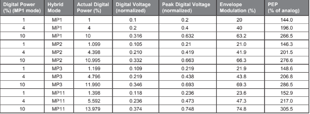
Table 1 sets out some of the more interesting numbers associated with 1 percent, 4 percent and 10 percent digital power injection levels. Intuitively, we might not think that 10 percent power would have a very big effect on anything, but it does. It all has to do with peak-to-average ratios, square roots and squares. These little mathematical operations conspire to produce some possibly surprising results.
Table 1 shows the power increase required for different digital power levels and hybrid and extended hybrid modes. MP1 mode uses 10 subcarrier partitions in each sideband. For extended hybrid modes, MP2 uses 11, MP3 uses 12 and MP11 uses 14. As the number of subcarriers increases, so does the digital power. In the extended hybrid modes, 10 percent digital power may increase to approximately 11 percent, 12 percent or 14 percent. However, power is not exactly proportional to the number of partitions (1.1, 1.2, or 1.4 times the MP1 power) because of the existence of one extra reference carrier per sideband.
Although Table 1 shows the effects of the extended hybrid modes (MP2 through MP11), the calculations, simulations and measurements in this paper are for the basic MP1 hybrid mode.

IBiquity’s peak-to-average ratio reduction system reduces the peaks to about 6 dB above the average digital power. This is a major improvement over no correction at all. When the vectors for n tones all line up in phase, the peak-to-average power ratio becomes simply n. For the 382 QPSK carriers (tones) this would be a peak-to-average ratio of 25.8 dB — but the probability level would be very low. Still, reducing it to 6 dB is a major improvement.
At 10 percent digital we have 63 percent AM and we need 53.3 kilowatts PEP for a 20 kilowatt analog signal. The ratio becomes even larger for the extended hybrid modes.
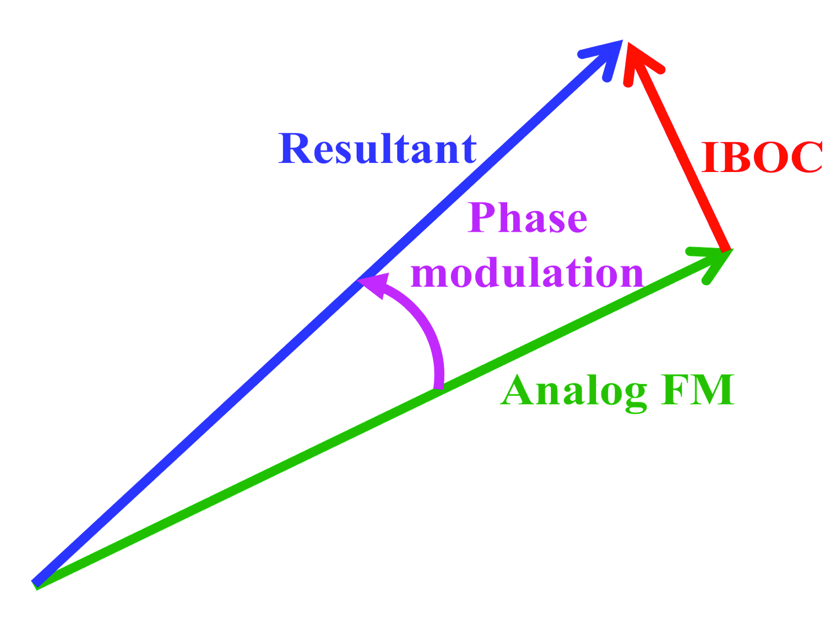
Fig. 1 shows what that 63 percent envelope modulation means. If we draw the analog FM signal as the black vector, and the digital signal is the red vector, then the blue vector shown in Fig. 1 is the resultant envelope at the negative modulation peaks. For 1 percent digital power we have about 20 percent AM. At the negative modulation troughs, we still have 80 percent of our signal to work with. The analog signal would have to fade 14 dB relative to the digital sidebands to pinch off the envelope. At 10 percent digital power, the envelope drops to 37 percent of normal on negative envelope peaks. That is only 4 dB of relative fading from pinch-off.
The danger for analog FM reception is that if the vector length goes to zero, the receiver produces noise bursts. Remember that an analog FM receiver contains a hard limiter (see Fig. 2). The hard limiter is a device whose gain is equal to the reciprocal of its input signal’s envelope. If the envelope goes to zero, an ideal limiter’s gain goes to infinity. A practical limiter will output noise bursts if its input envelope pinches off.
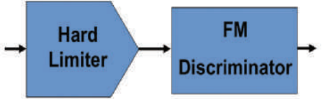
So, if there is a slight amount of multipath, causing only 4 dB of differential fading between the analog and digital components of a signal, the envelope at the receiver may pinch off, causing noise bursts on analog receivers. In other words, the digital signal may capture the analog FM demodulator.
This shows that peak-to-average ratio reduction is a good thing. Reducing positive modulation peaks significantly reduces transmitter PEP requirements. But reducing the negative envelope modulation improves the capture fade margin for the receivers.
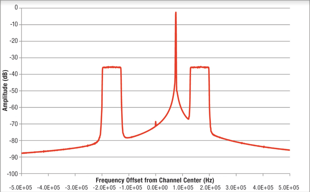
It could be argued that the digital sidebands are filtered out before the hard limiter, so there is no problem. This is true, to an extent. Unfortunately, the selectivity of IF filters are highly variable. Fig. 3 shows a plot of a typical FM bandpass filter made by Murata, with an IBOC spectrum superimposed on the same plot to the same scale. Murata makes monolithic ceramic bandpass filters used in many FM radios. They come in a variety of bandwidths. Electronically tuned car radios tend to have narrower bandwidths. Continuously tuned radios tend to have wider IF filters to make tuning less critical.
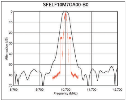
The filter shown in Fig. 3 has a nominal bandwidth of 230 kHz. It is a narrow type that might be used in a synthesized receiver. Careful inspection of the catalog curves show that the IBOC sidebands are reduced about 4 dB where they start and about 17 dB where they end. This is a good thing — if the sidebands can be reduced in amplitude before the hard limiter there is less danger of digital capture.
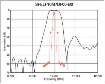
Fig. 4 shows one of Murata’s wider filters. This filter has a nominal bandwidth of 350 kHz. This one has negligible attenuation at the IBOC sidebands. So receivers with this kind of filter, which would give very good analog FM demodulation, are much more susceptible to differential fading multipath. Receivers with this kind of selectivity curve will get the full effect of the IBOC sidebands.
SELF-NOISE MECHANISMS
When an analog FM signal and IBOC sidebands are both present at a receiver’s demodulator, the IBOC sidebands produce a certain amount of phase modulation of the FM carrier. Fig. 5 shows an example at one instant in time. And the derivative of that phase modulation is the FM noise added by the IBOC sidebands.
It helps to look at the frequency domain when analyzing the effects of HD sidebands on the analog signal. We will start by looking at an unmodulated signal. FM demodulation is a highly nonlinear process.
In general, we cannot look at an RF spectrum and intuitively predict what will come out of an FM demodulator. However, when the modulation index is low enough, we can look at a spectrum and get an idea of where the first order phase modulation terms will appear. That is the case here — a low modulation index at high frequencies.

Fig. 6 shows the input to the demodulator with no modulation of the FM carrier. This results in a simple analysis. We can expect to see first-order phase modulation components beginning at 129 kHz and going up to 198 kHz. These components are due to the simple beat notes between the FM carrier and each one of the IBOC carriers. The FM stereo composite bandwidth is 53 kHz, so these first-order high-frequency components are out of band and will not be a problem to the demodulated stereo, unless the stereo demodulator responds to harmonics of 38 kHz.
Now imagine what happens if you modulate the analog with a very low frequency. Assume we are modulating 100 percent at 20 Hertz. The modulation is now so slow that we can think of it as a single carrier sweeping back and forth, from minus 75 kHz to plus 75 kHz. Fig. 7 shows what the carrier looks like when it hits a modulation peak. Now the beat notes have changed significantly. The lowest first-order beat is +75 kHz beating with +129 kHz. This produces a beat note of 54 kHz. Stereo L–R ends at 53 kHz. Analog overmodulation will clearly cause a problem with beat note products into the stereo baseband.
If we can imagine what comes out of the FM demodulator in this situation, we have a block of first-order beats that sweep back and forth from 54 up to 273 kHz, driven by the analog FM deviation. If this was all that came out of the FM demodulator, the analog signal with the possible exception of SCAs and RDS would be pristine.
But FM demodulation and the beat note generation process are quite nonlinear. The FM demodulation process takes derivatives of arctangent functions, which can make a real mess in the frequency domain.
SIMULATIONS
What follows are the results of some simulations. The simulations show what happens to the analog FM in the presence of different levels of HD injection, with different kinds of filtering and analog modulation.
First we begin with a FM+HD signal. Then we may filter the signal. The filter may simulate a receiver’s bandpass filter, multipath propagation, or both. Next the filtered FM+HD signal is applied to a “perfect” numerical FM demodulator. (See Fig. 8, showing a complex baseband simulation. The FM demodulator includes a hard limiter and produces as the demodulated FM.)

Finally, we do a spectrum analysis of what comes out of the FM demodulator. This allows us to see noise and distortion in the frequency domain.
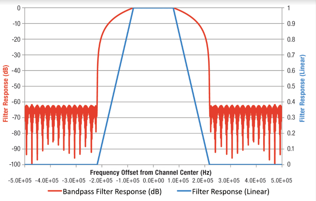
Some of the simulations we are about to see were done with full-blast IBOC power, with no bandwidth limiting. This simulates a wideband receiver. Simulations of a narrowband receiver were done with the linear phase FIR filter shown in Fig. 9, which closely approximates the amplitude response of the narrow Murata filter shown earlier. This filter slopes from –4 to –17 dB across the IBOC sideband blocks. The resulting attenuation of the IBOC sideband energy is 6.7 dB. So 10 percent digital power becomes 2.1 percent after this filter.
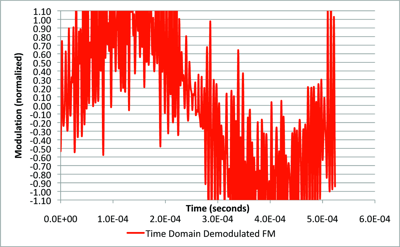
In a wide bandwidth, with no de-emphasis, Fig. 10 shows the time domain signal that comes out of the FM demodulator at 10 percent digital power. This is one cycle of 1.9 kHz mono, and the noise riding on it is due to the digital sidebands. This is a very scary picture, but fortunately the situation is not as bad as it looks.
We can insert the sharp IF filter to knock the IBOC sidebands down about 6.7 dB, and a post-detection 53 kHz brick-wall filter to limit the bandwidth to just the stereo composite baseband. These two measures get rid of the great majority of the unwanted FM. The waveform shown in Fig. 11 is not nearly as scary. All we see is a little bit of noise, mostly at the peaks of the sine wave.
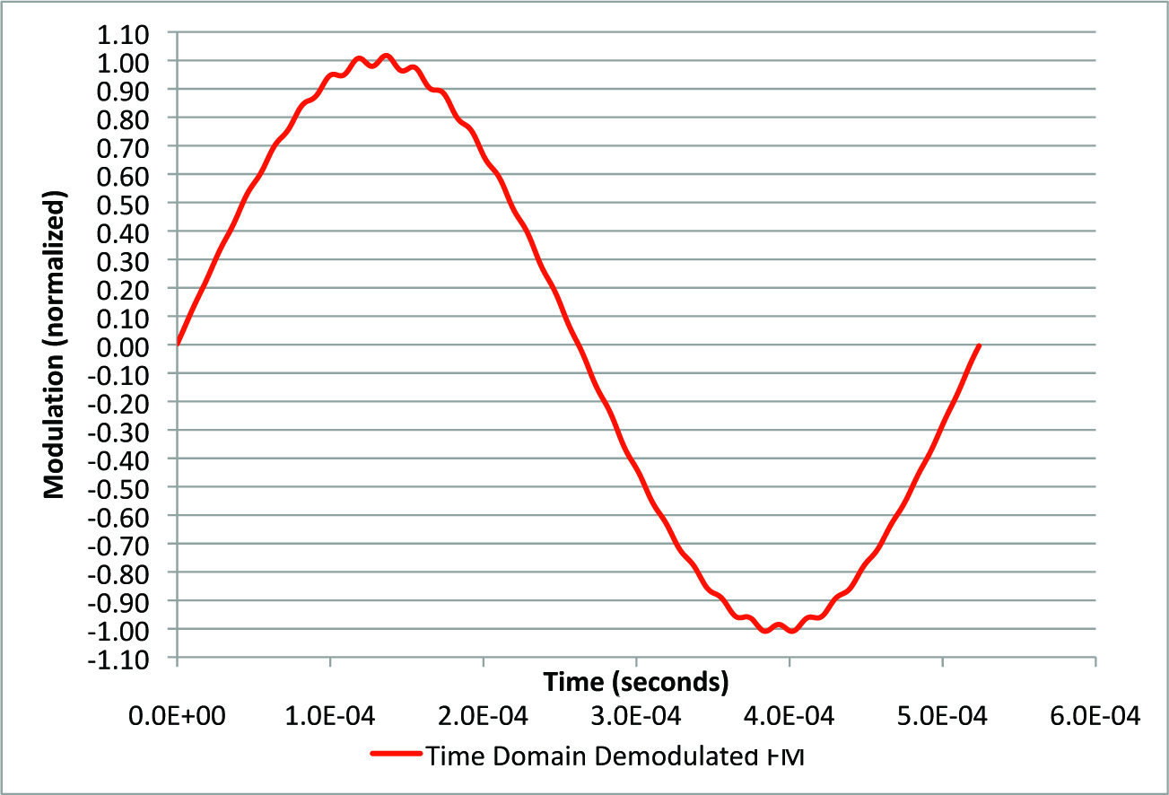
The noise appears mainly at the peaks, because those are the points where the carrier has deviated 75 kHz where it is much closer to the IBOC sidebands. So, the first-order beat notes are lower and they start to sneak inside the 53 kHz low-pass filter’s passband.
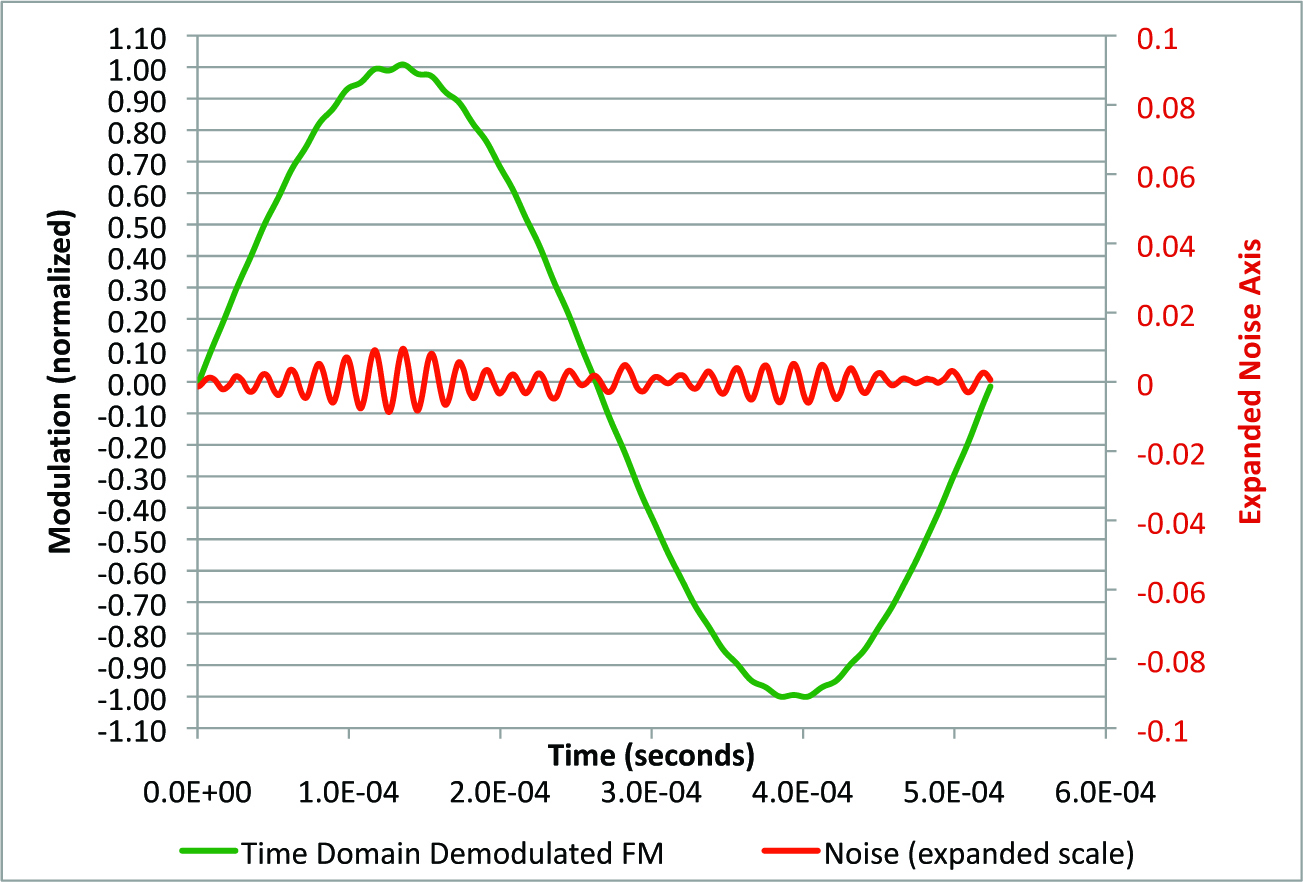
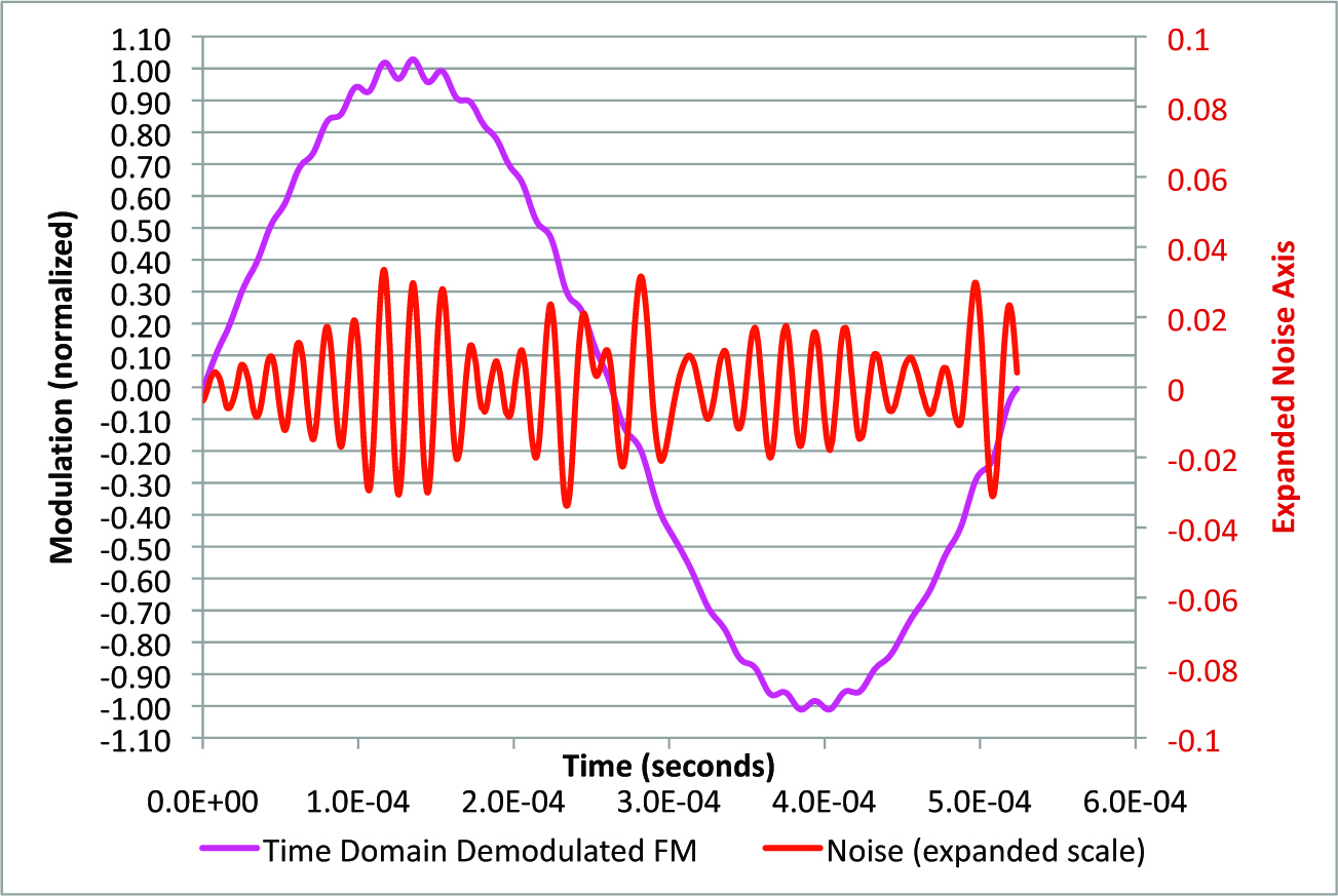
Now we can make a distortion analyzer numerically. Fig. 12 shows the FM detector output with 1 percent digital power with the brick-wall 53 kHz low-pass, but no IF filtering. The green trace is the demodulator output, and the red trace is the output of a notch filter that removes the 1.9 kHz fundamental tone. So the red trace is the demodulated noise. It is also shown on an expanded scale with a gain factor of about 10. Now we can clearly see the beat notes that get bigger as the sine wave reaches its peaks.
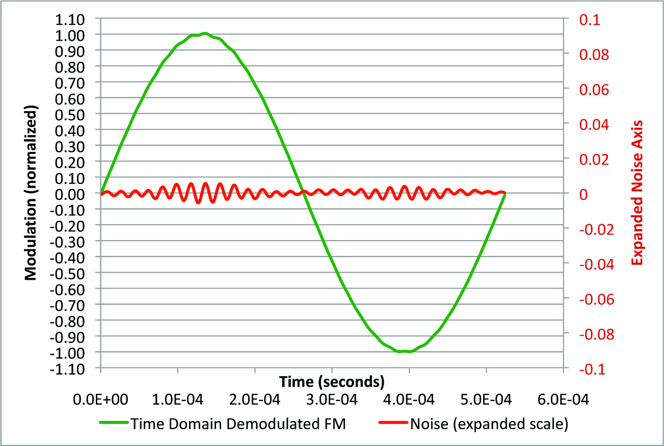
Fig. 13 shows what happens when we insert the sharp IF filter. The beat note is still present, but it is smaller.
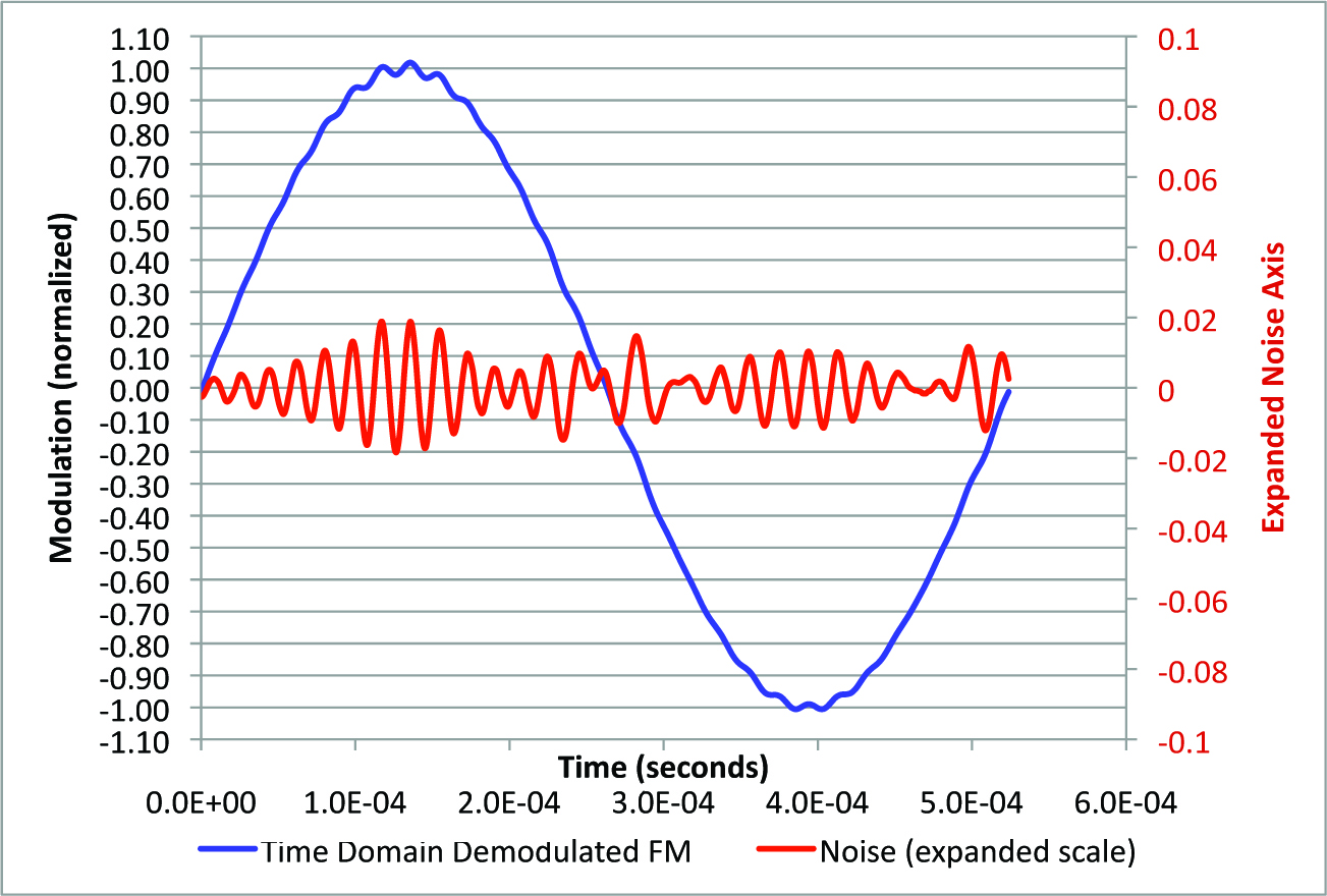
In Fig. 14 we have turned up the digital power to 4 percent. This is with no IF filtering, to simulate a wide bandwidth receiver. The noise is bigger.
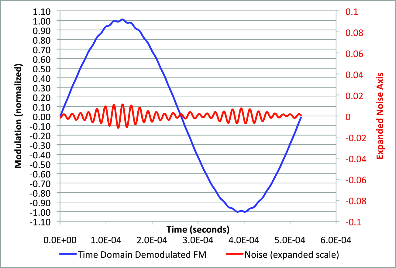
Fig. 15 shows 4 percent digital power with the sharp IF filter. As expected, the noise amplitude is reduced.
In Fig. 16 we have turned up the digital power to 10 percent. This is with no IF filtering, but the 53 kHz post-detection filter is still present. The noise is still bigger.
CONCLUSION
As has been shown, elevated digital power brings with it various engineering tradeoffs that raise concern. Higher digital power increases the amount of envelope modulation, reducing the amount of signal headroom at the demodulator. This will increase receiver susceptibility to noise bursts during multipath fading or even the possibility of “digital capture” of the receiver.
Additionally, as shown in the simulations, higher digital power results in increased intermodulation between the analog and digital signals, resulting in noise components in the stereo baseband area. This reduces the stereo signal-to-noise ratio on receivers, particularly on higher-quality models with wider IF bandwidths.
In Part II we will analyze the demodulated spectrum of elevated digital FM signals and quantify the signal to noise effects. Real-world tuner measurements will demonstrate the accuracy of the simulations. We will look at peak-to-average ratio reduction algorithms. Finally we will make some recommendations for evaluating elevated HD.
Contact author Dave Hershberger at [email protected].