Unless you are a hermit or a Stylite, robust interaction with your neighbors is usually a good thing. Of course, this is not the case with broadcast transmitters, where living in isolation is usually the preferred state.
Systems that start talking together are kind of like the neighbors on either side of you who party together and leave beer cans in your yard. Those guys are a nuisance, and so is the RF equivalent: intermodulation distortion, or more simply, intermodulation

This phenomenon has at its source the fact that we live in an imperfect world. In school, it was convenient to neglect air resistance and consider all systems as being linear. Unfortunately, it ain’t that way out here in the cold, and the actual non-linear nature of systems can cause multiple signals to combine and form transmitted products at new and undesired frequencies. These new products may land on frequencies used by other systems, and if high enough in magnitude, cause interference to other users.
Most times intermodulation products are created in a transmitter power amplifier, which is reasonable, given its active nature. IMD can also be created in receivers, and many times occurs in vintage radios or, in some cases, in the front end of a receiver pounded by high signal levels. In much less common cases, usually limited to ones where the field strength is high, metallic objects can act as a rectifier or mixer and create trash.
The late great Don Markley used to talk about a case where a spur created from the mix of two proximal FM stations was wreaking havoc on aircraft communications. Through direction finding techniques, he traced down the source of spur as being rusty fasteners on the siding of a communications shed. The kicker was the shed belonged to the FAA — the original complainant!

If we consider an amplifier that is perfectly linear and inject two signals at different frequencies, then our output will contain only those two original frequencies shifted only by amplitude and phase. The non-linear nature of devices allows for the creation of the additional products. In the simplest case of intermodulation, non-linear conditions create harmonics, which are integral multiples of a single fundamental frequency. Most transmitters will have a filtering scheme to reduce the level of these products of which the second and third are usually the most egregious.
As the quantity of signals increases, the number of potential products increases as well. Products are referred to by “order,” which is the sum of the absolute values of the coefficients of the fundamental frequencies.
As an example, the product of twice one frequency minus the other is third order. Similarly, an example of a fifth order product is three times one frequency minus twice the other.

Note that as the order increases, the probability of a given product decreases, as amplifier harmonics typically decrease in magnitude as their frequency increase. Although the probability of a seventh or higher order product occurring is non-zero, it is very small.
To see how the number of potential products spirals upward, consider a site with two FM stations. The number of potential third, fifth, and seventh order products are 12, 30 and 56, respectively. Increase the number of stations by one, and the result is 31, 114 and 286 products, respectively. Make it four stations, and now you are at 64, 337 and 1,115 potential products.
At large communications sites, the number of potential products can easily be in the thousands. Of course, not all products will be there and consideration of modulation types, equipment design and frequency separation factor into the potential of a given product. While a microwave and AM transmitter creating a spur is possible, if you find one of these actually occurring, I would suggest buying Powerball tickets.
FILTERING
In the event that products are found to exist, no equipment issues are present, and the cause of products is outside frequencies coupling through the antenna system, the typical way of elimination or reduction is through filtering.


Filtering reduces the magnitude of outside signals reaching the device, thereby reducing the magnitude of products created in the amplifier. Products transmitted also travel through the filter and are therefore reduced in magnitude.
Four basic filter topologies exist, and the utility of each depends on the source and frequency of the signals involved.
In a case where two FM stations are potentially mixing, a band reject in the form of a notch in the path of each may be sufficient. The use of notch filters becomes impractical and costly if a greater number of signals are involved as each external frequency entering a device requires its own notch. Low pass or high pass filters may be appropriate in cases where the frequencies are disparate. Ultimately, the best solution is probably a band pass filter centered on the desired transmit frequency. Such filters can be thought of as high pass filter cascaded through a low pass filter.
FIND THE SOURCE
If the location of a generator of an undesirable product is unknown, direction-finding techniques will be necessary. Triangulation of the source location can usually be made through successive iterations of identifying a peak azimuth from various locations in a circle around the source and plotting them on a map. If the horizontal plane pattern of the receive antenna is broad, it may be necessary to triangulate multiple times to converge on a location, while moving closer to the apparent source each time.
When the source is finally determined, it is desirable to establish the level of the products to determine compliance with the commission’s rules, or lack thereof. A spectrum analyzer, filter assortment and sample method is the equipment set of choice. Filters are important to ensure that the fundamental frequencies are sufficiently reduced not only to provide sufficient dynamic range, but also to ensure that other spurious products are not generated in the front end of the analyzer.
Filters and cable assemblies must be accurately characterized at the frequencies under consideration in order to derive correction factors for their responses. Depending on the methodology utilized, additional correction factors may be required for the sample apparatus, as well. Transmission line sections that use removable plug-in sample slugs can be assumed, based on manufacturer literature, to have a flat response across their specified operational range. Directional couplers, however, typically have a frequency-dependent coupling value. Variations in the coupling value can induce inaccuracies into measurements, especially those that diverge from the fundamental by a significant amount such as harmonics and higher order products.

Ideally, the frequency response of a directional coupler should be fully determined across the entire spectrum under consideration. If this data is not available, or cannot be acquired, then the assumption must be made that the coupler will provide a sample that increases in magnitude by 6 dB per octave. In other words, a measured second harmonic, which is twice the frequency of the fundamental, will be 6 dB higher than the actual sample or level being “transmitted.” The third harmonic will be 9 dB lower than measured, the fourth 12 dB lower, and so on.
The ideal equipment for characterizing and tuning filters and other apparatus is a two-port network analyzer.
Once the measured levels are determined and appropriate corrections for cables, filters and other components made, the actual value relative to the fundamental carrier should be checked to ensure rule compliance. The two sections pertinent to radio broadcasters are 73.44 for AM stations and 73.317 for FM stations. In each case, the emission limits are frequency based relative to the carrier.
For AM stations, the emission limitations form the familiar NRSC mask and vary with frequency. Closer to the carrier the attenuation limits are lower, reaching -65 dBc in the range removed 60-75 kHz from the carrier. Beyond 75 kHz from the carrier, products must be attenuated to at least -65 dBc for transmitter powers of 158 Watts or less. Above this threshold, the attenuation level is the lesser of -80 dBc or 43 plus ten-times the base-10 logarithm of the power in Watts. Good practice is to shoot for 80 dB down, and if it is not achieved, run the calculation and see if compliance is achieved. The 80 dB figure is based on transmitter powers of at least 5 kW, so lower transmitter powers will allow for a lower attenuation level.
In the case of FM stations, the attenuation required is -25 dBc in the 120-240 kHz from carrier range, -35 dBc in the 240-600 kHz from carrier range, and beyond 60 kHz out, the familiar 43 plus ten-time the base-10 logarithm of the transmitter becomes relevant. As was the case with AM systems, the attenuation level is the lesser of this value and -80 dBc. It is important to note that even signals attenuated well below these levels can cause problems to other users, namely LTE uplinks. In that case, and others, filtering may require the addition of shielding to keep the neighbors happy.
Identification and elimination of intermodulation products is usually straightforward, although every once in a while, a curve ball is thrown that challenges the acumen of the most astute engineer. In such cases, a combination of elimination theory and Occam’s Razor will usually get you to the answer, and more importantly, get the beer cans out of the yard.